Roses Are Red Violets Are Blue if I Were a Null Hypothesis Id Fail to Reject You
- Hypothesis Testing
- Hypothesis testing is an inferential procedure that uses sample data to evaluate the credibility of a hypothesis about a population.
- The Logic of Hypothesis Testing
- Put simply, the logic underlying the statistical hypothesis testing procedure is:
- State the Hypothesis: We state a hypothesis (guess) about a population. Usually the hypothesis concerns the value of a population parameter.
- Define the Decision Method: We define a method to make a decision about the hypothesis. The method involves sample data.
- Gather Data: We obtain a random sample from the population.
- Make a Decision: We compare the sample data with the hypothesis about the population. Usually we compare the value of a statistic computed from the sample data with the hypothesized value of the population parameter.
- If the data are consistent with the hypothesis we conclude that the hypothesis is reasonable.
- If there is a big discrepency between the data and the hypothesis we conclude that the hypothesis was wrong.
- Errors in Hypothesis Testing
- The purpose of hypothesis testing is to make a decision in the face of uncertainty. We do not have a fool-proof method for doing this: Errors can be made. Specifically, two kinds of errors can be made:
- Type I Error: We decide to reject the null hypothesis when it is true.
- Type II Error: We decide not to reject the null hypothesis when it is false.
- Hypothesis Testing Techniques
- We present the technical aspects of the steps later in these notes. This part covers non-directional (two-tailed) techniques which are appropriate when the experimenter predicts an effect, but doesn't predict the direction of the effect.
- Directional Hypothesis Testing
- Directional (One-Tailed) tests are used when the experimenter predicts a direction of the effect.
- Power of Hypothesis Testing
- The power of a hypothesis test is discussed in the last section of these notes.
- First Step: State the hypothesis
Stating the hypothesis actually involves stating two opposing hypotheses about the value of a population parameter.Example: Suppose we have are interested in the effect of prenatal exposure of alcohol on the birth weight of rats. Also, suppose that we know that the mean birth weight of the population of untreated lab rats is 18 grams.
Here are the two opposing hypotheses:
- The Null Hypothesis (Ho). This hypothesis states that the treatment has no effect. For our example, we formally state:
The null hypothesis (Ho) is that prenatal exposure to alcohol has no effect on the birth weight for the population of lab rats. The birthweight will be equal to 18 grams. This is denoted

- The Alternative Hypothesis (H1). This hypothesis states that the treatment does have an effect. For our example, we formally state:
The alternative hypothesis (H1) is that prenatal exposure to alcohol has an effect on the birth weight for the population of lab rats. The birthweight will be different than 18 grams. This is denoted

- The Null Hypothesis (Ho). This hypothesis states that the treatment has no effect. For our example, we formally state:
- Second Step: Set the Criteria for a decision.
The researcher will be gathering data from a sample taken from the population to evaluate the credibility of the null hypothesis.A criterion must be set to decide whether the kind of data we get is different from what we would expect under the null hypothesis.
Specifically, we must set a criterion about wether the sample mean is different from the hypothesized population mean. The criterion will let us conclude whether (reject null hypothesis) or not (accept null hypothesis) the treatment (prenatal alcohol) has an effect (on birth weight).
We will go into details later.
- Third Step: Collect Sample Data.
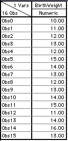
Now we gather data. We do this by obtaining a random sample from the population.Example: A random sample of rats receives daily doses of alcohol during pregnancy. At birth, we measure the weight of the sample of newborn rats. We calculate the mean birth weight.
- Fourth Step: Evaluate the Null Hypothesis
We compare the sample mean with the hypothesis about the population mean.- If the data are consistent with the hypothesis we conclude that the hypothesis is reasonable.
- If there is a big discrepency between the data and the hypothesis we conclude that the hypothesis was wrong.
Example: We compare the observed mean birth weight with the hypothesized values of 18 grams.
- If a sample of rat pups which were exposed to prenatal alcohol has a birth weight very near 18 grams we conclude that the treatement does not have an effect. Formally we do not reject the null hypothesis.
- If our sample of rat pups has a birth weight very different from 18 grams we conclude that the treatement does have an effect. Formally we reject the null hypothesis.
In the second step of the procedure we identify the kind of data that is expected if the null hypothesis is true. Specifically, we identify the mean we expect if the null hypothesis is true.
If the outcome of the experiment is consistent with the null hypothesis, we believe it is true (we "accept the null hypothesis"). And, if the outcome is inconsistent with the null hypothesis, we decide it is not true (we "reject the null hypothesis").
We can be wrong in either decision we reach. Since there are two decisions, there are two ways to be wrong.
| Errors in Hypothesis Testing | ||||||||||||
|---|---|---|---|---|---|---|---|---|---|---|---|---|
| ||||||||||||
- Type I Error: A type I error consists of rejecting the null hypothesis when it is actually true. This is a very serious error that we want to seldomly make. We don't want to be very likely to conclude the experiment had an effect when it didn't.
The experimental results look really different than we expect according to the null hypothesis. But it could come out the way it did just because by chance we have a wierd sample.
Example:We observe that the rat pups are really heavy and conclude that prenatal exposure to alcohol has an effect even though it doesn't really. (We conclude, erroneously, that the alcohol causes heavier pups!) There could be for another reason. Perhaps the mother has unusual genes.
- Type II Error: A type II error consists of failing to reject the null hypothesis when it is actually false. This error has less grevious implications, so we are will to err in this direction (of not concluding the experiment had an effect when it, in fact, did).
The experimental results don't look different than we expect according to the null hypothesis, but they are, perhaps because the effect isn't very big.
Example: The rat pups weigh 17.9 grams and we conclude there is no effect. But "really" (if we only knew!) alcohol does reduce weight, we just don't have a big enough effect to see it.
The techniques of hypothesis testing allow us to know the probability of making a type I error.
We do this by comparing the sample mean  and the population mean hypothesized under the null hypothesis
  and decide if they are "significantly different". If we decide that they are significantly different, we reject the null hypothesis that
  .
.
To do this we must determine what data would be expected if Ho were true, and what data would be unlikely if Ho were true. This is done by looking at the distribution of all possible outcomes, if Ho were true. Since we usually are concerned about the mean, we usually look at the distribution of sample means for samples of size n that we would obtain if Ho were true.
Thus, if we are concerned about means we:
- Assume that Ho is true
- Divide the distribution of sample means into two parts:
- Those sample means that are likely to be obtained if Ho is true.
- Those sample means that are unlikely to be obtained if Ho is true.
 . Thus:
  = the probability of a Type I error.
By convention, we usually adopt a cutoff point of either:
 or
or  or occasionally
  .
.
If we adopt a cutoff point of
-

- then we know that the obtained sample of data is likely to be obtained in less than 5 of 100 samples, if the data were sampled from the population in which Ho is true.
We decide: "The data (and its sample mean) are significantly different than the value of the mean hypothesized under the null hypothesis, at the .05 level of significance."
This decision is likely to be wrong (Type I error) 5 times out of 100. Thus, the probability of a type I error is .05.
-

- The obtained sample of data is likely to be obtained in less than 1 of 100 samples, if the data were sampled from the population in which Ho is true.
We decide: "The data (and its sample mean) are significantly different than the value of the mean hypothesized under the null hypothesis, at the .01 level of significance."
This decision is likely to be wrong (Type I error) 1 time out of 100. Thus, the probability of a type I error is .05.
-

- The obtained sample of data is likely to be obtained in less than 1 of 1000 samples, if the data were sampled from the population in which Ho is true.
We decide: "The data (and its sample mean) are significantly different than the value of the mean hypothesized under the null hypothesis, at the .001 level of significance."
This decision is likely to be wrong (Type I error) 1 time out of 1000. Thus, the probability of a type I error is .05.
 Example: We return to the example concerning prenatal exposure to alcohol on birth weight in rats. Lets assume that the researcher's sample has n=16 rat pups. We continue to assume that population of normal rats has a mean of 18 grams with a standard deviation of 4.
There are four steps involved in hypothesis testing:
- State the Hypotheses:
- Set the decision criteria:
- Gather Data:
Lets say that two experimenters carry out the experiment, and they get these data:Experiment 1 Experiment 2 

Experiment 1 Experiment 2 Sample Mean = 13 Sample Mean = 16.5 - Evaluate Null Hypothesis:
We calculate Z for each experiment, and then look up the P value for the obtained Z, and make a decision. Here's what happens for each experiment:Experiment 1 Experiment 2 Sample Mean = 13
Z = (13-18)/1 = -5.0
p < .0000
Reject Ho
ViSta AppletSample Mean = 16.5
Z = (16.5-18)/1 = -1.5
p = .1339
Do Not Reject Ho
ViSta AppletViSta's Report for Univariate Analysis of Experiment 1 Data. 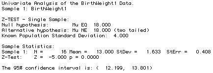
ViSta's Report for Univariate Analysis of Experiment 1 Data. 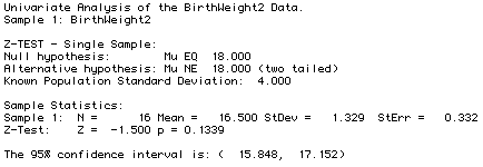
- Non-directional (Two-Tailed) Hypothesis
- The statistical hypotheses (Ho and H1) specify a change in the population mean score.
In this section we can consider directional, "One-Tailed", hypothesis testing. This is what is used when the experimenter expects a change in a specified direction.
- Directional (One-Tailed) Hypothesis
- The statistical hypotheses (Ho and H1) specify either an increase or a decrease in the population mean score.
Example: We return to the survey data that we obtained on the first day of class. Recall that our sample has n=41 students.
| Sample Statistics, Population Parameters and Sample Frequency Distribution for SAT Math | |
|---|---|
| Statistics & Parameters | Sample Frequency Distribution |
| Sample Statistics Samp. Mean = 589.39 Samp. Stand. Dev. = 94.35 | |
| Population Parameters Pop. Mean = 460 Pop. Stand. Dev. = 100 | |
Note that red is for males, blue for females.
The same four steps are involved in both directional and non-directional hypothesis testing. However, some details are different. Here is what we do for directional hypothesis testing:
- State the Hypotheses:
- Alternative Hypothesis: Students in this class are sampled from a restricted selection population whose SAT Math Scores are above the unrestricted population's mean of 460. There is a restrictive selection process for admitting students to UNC that results in SAT Math scores above the mean: Their mean SAT score is greater than 460.
- Null hypothesis: Students in this class are not sampled from a restricted selection population whose SAT Math Scores are above the unrestricted population's mean of 460. There is an unrestrictive selection process for admitting students to UNC: Their mean SAT score is not greater than 460.
- Symbols:

- Set the decision criteria:
- Gather Data:
We gathered the data on the first day of class and observed that the class's mean on SAT Math was 589.39. - Evaluate Null Hypothesis:
We calculate Z and then look up the P value for the obtained Z, and make a decision. Here's what happens:

The P value is way below .00001, so we reject the null hypothesis that there is an unrestrictive selection process for admitting students to UNC. We conclude that the selection process results in Math SAT scores for UNC students that are higher than the population as a whole.Try the ViSta Applet for carrying out this analysis. You should get the following report.
ViSta's Report for Univariate Analysis of SAT Math Scores. 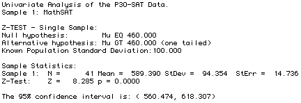
We have examined the potential for making an incorrect decision, looking at Type I and Type II errors, and the associated signicance level for making a Type I error.
We now reverse our focus and look at the potential for making a correct decision. This is refered to as the power of a statistical test.
- Statistical Power
- The power of a statistical test is the probability that the test will correctly reject a false null hypothesis. The more powerful the test is, the more likely it is to detect a treatment effect when one really exists.
- Power and Type II errors:
- When a treatment effect really exists the hypothesis test:
- can fail to discover the treatment effect (making a Type II error). The probability of this happening is denoted:
 = P[Type II error]
 - can correctly detect the treatment effect (rejecting a false null hypothesis). The probabililty of this happening, which is the power of the test, is denoted:
 = power = P[rejecting a false Ho].
- can fail to discover the treatment effect (making a Type II error). The probability of this happening is denoted:
Here is a table summarizing the Power and Significance of a test and their relationship to Type I and II errors and to "alpha" and "beta" the probabilities of a Type I and Type II error, respectively:
| Decisions in Hypothesis Testing | ||||||||||||
|---|---|---|---|---|---|---|---|---|---|---|---|---|
| ||||||||||||
- How to we determine power?
- Unfortunately, we don't know "beta", the exact value of the power of a test. We do know, however, that the power of a test is effected by:
- Alpha Level: Reducing the value of alpha also reduces the power. So if we wish to be less likely to make a type I error (conclude there is an effect when there isn't) we are also less likely to see an effect when there is one.
- One-Tailed Tests: One tailed tests are more powerful. They make it easier to reject null hypotheses.
- Sample Size: Larger samples are better, period. Tests based on larger samples are more powerful and are less likely to lead to mistaken conclusions, including both Type I and Type II errors.
Source: https://www.uv.es/visualstats/vista-frames/help/lecturenotes/lecture07/hyptest97.html


0 Response to "Roses Are Red Violets Are Blue if I Were a Null Hypothesis Id Fail to Reject You"
Post a Comment